

Profit and loss (P&L) explain, also called P&L attribution, identifies the drivers of a change in portfolio value. It should show what changed, estimate each driver's contribution, and reconcile those contributions to the actual change.
This article describes how MASTIX Derivatives Studio handles P&L explain for the change in modeled portfolio value between two valuation states. It connects valuation, configured market sensitivities, and attribution in one analytical workflow. Any difference not explained by the attributed components remains visible as residual P&L.
Accounting or desk P&L may also include realized cash, fees, funding, reserves, ledger adjustments, or other items outside that modeled value change.
What a P&L explain separates
The explain starts with three primary components:
- Portfolio composition: new, closed, matured, or amended positions
- Time effects: cash flows, fixings, discounting, and the passage of time
- Market data: movements in curves, benchmark quotes, and other configured factors
Where implemented, model and assumption changes can be reported separately.
The attributed components are reconciled to the actual change in portfolio value. Any remaining difference is reported as residual P&L.
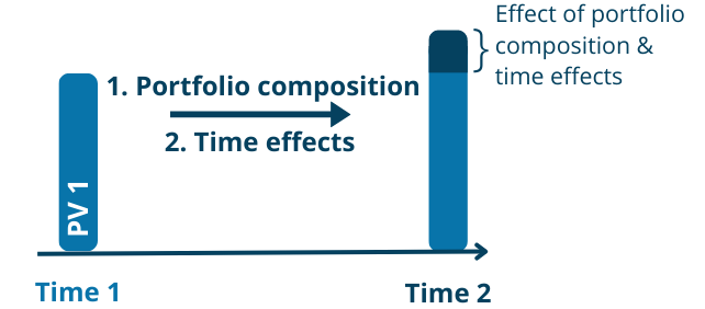
Figure 1: Portfolio composition and time effects.
Sensitivities explain market-data effects
One way to explain market-driven P&L is through benchmark quotes and the portfolio's sensitivities to them.
For each configured risk factor, the contribution is approximated as:
Estimated contribution: sensitivity × quote move
The contributions are aggregated across the configured sensitivity set. This connects observed market moves to their estimated effect on portfolio value.
The result depends on:
- coverage of the portfolio's material risk factors
- consistent quote, curve, and benchmark definitions
- consistent position snapshots and valuation assumptions
- the size and nonlinearity of the market move
Missing factors, cross-factor interactions, nonlinear effects, and inconsistent inputs remain in the residual unless handled by a separate refinement.
AAD avoids factor-by-factor reruns
A standard way to calculate sensitivities is bump-and-revalue:
- shift one market input
- rerun the valuation
- measure the change
- repeat for each factor
The number of valuation runs grows with the factor set.
Derivatives Studio uses Adjoint Algorithmic Differentiation (AAD) to calculate derivatives of implemented valuation functions with respect to configured inputs. For supported instruments and risk factors, it produces the configured first-order sensitivity set without a separate portfolio rerun for each factor.
This has three practical effects:
- valuation and sensitivities use the same implemented analytical definitions
- fewer valuation runs are required
- sensitivities remain linked to the calculation used for attribution
AAD covers the market sensitivity calculation, not the full explain. Portfolio activity and time effects still require consistent input states, and market attribution still depends on factor coverage and the attribution method.
Refining attribution with a fitted polynomial
A first-order explain holds sensitivity constant over a quote move. Derivatives Studio refines the estimate by fitting a second-order polynomial using the available portfolio values and derivatives.
The fitted polynomial is then used to extrapolate the value change from q₁ over the quote move. This captures curvature that a constant-delta approximation misses while keeping the calculation within the same sensitivity-based framework.
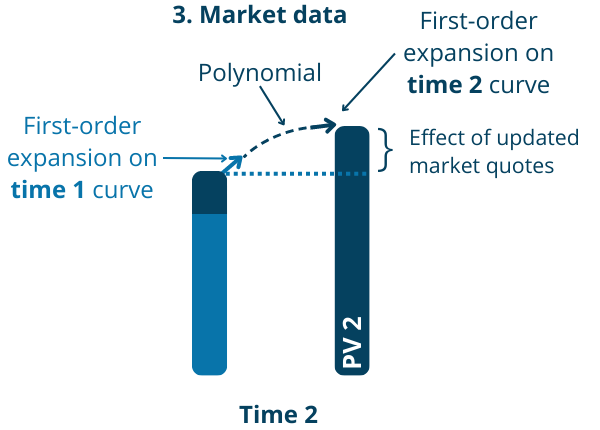
Figure 2: Updated market data and delta interpolation.
The fitted polynomial captures curvature in each risk factor separately. It does not include mixed cross-factor terms, so cross-factor interactions remain in the residual. Discontinuities, factors outside the configured set, and inconsistent inputs also remain unexplained.
P&L explain in practice
A configured Derivatives Studio attribution compares two states containing positions, market data, and valuation inputs. The output shows:
- which inputs changed
- the size of each change
- the estimated contribution to portfolio value
- the residual between the attributed components and the actual value change
Users can investigate results in the Excel add-in or integrate the analysis through the API.
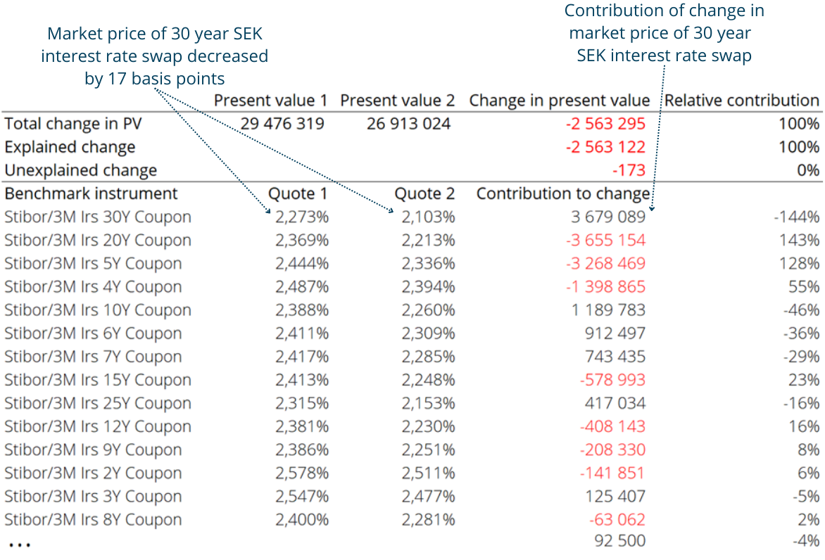
Figure 3: Example attribution output for the present value of a portfolio of interest rate swaps. Only the first benchmark instruments are shown.
Applying the method to VaR scenarios
The same sensitivity-based decomposition can be applied to an individual market scenario within a Value at Risk (VaR) framework. The observed daily moves are replaced by the factor moves in the scenario, allowing its estimated P&L to be separated by driver.
This explains the P&L of that scenario. It is not, by itself, an allocation of the VaR statistic. Scenario generation, confidence level, holding period, quantile selection, aggregation, and governance belong to the surrounding VaR methodology.
From P&L to its drivers
Derivatives Studio keeps the attributed components linked to the valuation and reports any unexplained amount as residual P&L.
AAD avoids one valuation rerun per configured first-order factor. Analysts can move from a result to its drivers without rebuilding the explanation from separate calculations.